Visualizing the Sutherland Hodgman algorithm

A Collision Detection System uses the GJK algorithm to determine if two polygons have collided. Unfortunately, the GJK algorithm does not provide the location of the collision. That is, it does not provide the Contact Manifolds (Contact Points) of the collision. Fortunately, the Sutherland-Hodgman algorithm does provide this information, and game engines use the Sutherland-Hodgman algorithm (after a collision is detected) to compute the collision response between two game characters.

Point distance to Plane

The Sutherland-Hodgman algorithm requires the distance between a point and a plane to apply its Clipping Rule. However, only the sign of the distance is necessary. If the distance between a point and a plane is positive, the point is considered to be on the Front side of the plane. If the distance is negative, the point is said to be on the Back side of the plane.

Sutherland-Hodgman Overview

Before we work through an example, let me give you a brief overview of how the algorithm works. Assume a collision between two square polygons. The algorithm starts by identifying a Reference and an Incident Polygon.

The segments of the Reference Polygon serve as Reference Planes for the algorithm. In our example, there are four reference planes. (In 2D a plane is a line.)

Once a reference polygon is identified, the algorithm tests each vertex of the Incident Polygon against each reference plane.

And it applies the following rule:

Sutherland-Hodgman Clipping Rule

• If points P1 and P2 are on the front side of the plane, the algorithm saves point P2.
• If points P1 and P2 are on the back side of the plane, then none of the points are saved.
• If P1 is on the front and P2 is on the back side of the plane, then compute an intersection point with the plane. The algorithm stores the intersection point.
• If P1 is on the back side and P2 is on the front side of the plane, the compute an intersection point with the plane. The algorithm stores point P2 and the intersection point.

The algorithm terminates by generating a new polygon whose vertices are the contact points of two collided polygons.

Sutherland-Hodgman in 2D

Let's go through an example in 2D.

1) Assume two boxes are interpenetrating. The first step is to identify the reference and the incident polygon.

2) For each reference plane, apply the Sutherland-Hodgman Clipping rule.

2a) Starting with the left plane (see image below):

• In the first instance, both points P1 & P2 are in front of the plane. Thus, P2 is saved.
• In the second instance, both points are in front of the plane which leads to P2 being saved.
• In the third case, both points are in front of the plane. Thus, P2 is stored.
• Finally, the last example shows both points in front of the plane. P2 is saved.

The algorithm uses these collected points to generate a new polygon. This new polygon is used as the input for the next iteration.

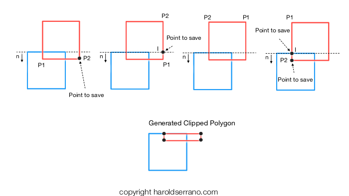
2b) Using the generated polygon and the next reference plane, apply the Sutherland-Hodgman Clipping rule again.

• In the first instance, both P1 & P2 are in front of the plane. Thus, P2 is saved.
• In the second case, P1 is in front of the plane, but P2 is on the back of the plane. According to the rule, an intersection point with the plane is calculated. This intersection point is saved.
• During the third instance, both P1 & P2 are on the back of the plane. Thus, none of these points are saved.
• Finally, in the fourth example, P1 is on the back of the plane and P2 is in front of the plane. An intersection point is calculated. Both P2 and the intersection point are saved.

The algorithm creates a new polygon from these new points.

2c) Using the previously generated polygon, repeat the Sutherland-Hodgman algorithm to the right reference plane.

• In the first case, P1 is in front of the plane and P2 is on the back. Thus, an intersection point is calculated and saved.
• In the second instance, no points are saved since they both lie on the back of the plane.
• In the third example, P1 is on the back and P2 is in front of the plane. An intersection point is calculated and saved along with P2.
• In the fourth instance, both P1 & P2 are in front of the plane. According to the rule, only P2 is saved.

The algorithm creates a new polygon using these stored points. This polygon is used as the input to the next iteration of the algorithm.

2d) Repeat the process with the last reference plane.

• In every instance, the points lie in front of the plane. Thus, the four corresponding points, P2, are saved.

3) The algorithm terminates generating a new polygon whose vertices represent the contact points of the collision.

Sutherland-Hodgman in 3D

The Sutherland-Hodgman algorithm is also employed to detect the contact points in a 3D collision. Even though the GJK does not provide contact manifolds, it does provide the following information:

• Collision Normal vector.
• Closest Collision Point between objects.

These two bits of information are used to create a Collision Plane. (If you recall, a plane is defined by a Normal vector and a point). The faces of the colliding polygons are then projected onto this plane. And it essentially turns a 3D Sutherland-Hodgman problem into a 2D Sutherland-Hodgman problem (as shown above).

For example,

1) Assume two cubes colliding. The GJK provides a Collision Normal vector and Closest Collision Point.

2) Calculate a Collision Plane using the Normal vector and the Closest point.

3) The closest (and most parallel) faces of each polygon are projected onto the Collision Plane:

4) The Sutherland-Hodgman algorithm is applied in 2D space. The vertices of the generated polygon represent the contact points of the collision.

Hope this helps.