Applying Light to a 3D model using Metal

In the previous post, you learned how to shade a 3D model. The shading effect was very simple. It merely provided the 3D model with a depth-perception. In this post, you will learn how to light an object by simulating Ambient-Diffuse-Specular (ADS) Lighting.

Before I start, I recommend you to read the prerequisite materials listed below:

Prerequisite:

How Light Works?

When light rays hit an object, the rays are either reflected, absorbed or transmitted. For our discussion, I will focus solely on light rays reflection.

When a light ray hits a smooth surface, the ray will be reflected at an angle equal to its incident ray. This type of reflection is known as Specular Reflection.

Visually, specular reflection is the white highlight seen on smooth, shiny objects.

In contrast, when a light ray hits a rough surface, the ray will be reflected at a different angle as its incident ray. This type of reflection is known as Diffuse Reflection.

Diffuse reflection enables our brain to make out the shape and the color of an object. Thus, diffuse reflection is more important to our vision than specular reflection.

Let's go through a simple animation to understand the difference between these reflections.

The animation below shows a 3D model with only specular reflection:

Whereas, the animation below shows a 3D model with only diffuse reflection:

As you can see, it is almost impossible for our brain to make out the shape of an object with only specular reflection.

There is another type of reflection known as Ambient Reflection. Ambient reflection is light rays that enter a room and bounces multiple types before reflecting off a particular object.

When we combine these three types of reflections, we get the following result:

Simulating Light Reflections

Now that you know how light works, the next question is: How can we model it mathematically?

Diffuse Reflection

In diffuse reflection, a light ray's reflection angle is not equal to its incident angle. From experience, we also know that a light ray's incident angle influences the brightness of an object. For example, an object will have different brightness when a light ray hits the object's surface at a 90-degree angle than when light rays hit the surface at a 5-degrees angle.

Mathematically, we can simulate this natural behavior by computing the Dot-Product between the light rays and a surface's Normal vector. When a light source vector S is parallel and heading in the same direction as the normal vector n, the dot product is 1, meaning that the surface location is fully lit. Recall, the dot product ranges between [-1.0,1.0].

As the light source moves, the angle between vectors S and n changes, thus changing the dot product value. When this occurs, the brightness levels also changes.

Taking into account the surface's Diffuse Reflection factor, the equation for Diffuse Reflection is:

diffuseEquation.png

Specular Reflection

In Specular Reflection, the light ray's reflection angle is always equal to its incident angle. However, the specular reflection that reaches your eyes is dependent on the angle between the reflection ray (r) and the viewer's location (v).

This behavior implies that to model a specular reflection; we need to compute a reflection vector from a normal vector and the light ray vector. We then calculate the influence of the reflection's vector onto the viewer's vector, i.e., we compute the dot product. The result provides the specular reflection of the object.

Taking into account the surface's Specular Reflection factor, the equation for Specular Reflection is:

The exponent determines the size of the highlight.

Ambient Reflection

There is not much to ambient reflection. The ambient reflection depends on the light’s ambient color and the ambient’s material reflection factor.

The equation for Ambient Reflection is:

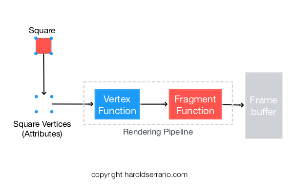
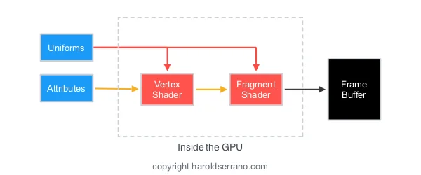
Simulating Light in the Rendering Pipeline

In Computer Graphics, Light is simulated in either the Vertex or Fragment Shaders. When lighting is simulated in the Vertex Shader, it is known as Gouraud Shading. If lighting is simulated in the Fragment Shader, it is known as Phong Shading.

Gouraud shading (AKA Smooth Shading) is a per-vertex color computation. What this means is that the vertex shader determines the lighting for each vertex and pass the lighting results, i.e. a color, to the fragment shader. Since this color is passed to the fragment shader, it is interpolated across the fragments thus giving the smooth shading.

Here is an illustration of the Gouraud Shading:

In contrast, Phong shading is a per-fragment color computation. The vertex shader provides the normal vectors and position data to the fragment shader. The fragment shader then interpolates these variables and calculates the lighting for the fragment.

Here is an illustration of the Phong Shading:

With either, Gouraud or Phong Shading, the Lighting computation is the same, although the results will differ.

In this project, we will implement a Phong Shading Light effect. For your convenience, I provide link to the Gouraud Shading Light project at the end of the article.

Setting up the project

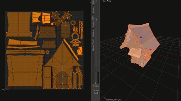
Let's apply Lighting (Phong shading) to a 3D model.

By now, you should know how to set up a Metal Application and how to implement simple shading to a 3D object. If you do not, please read the prerequisite articles mentioned above.

For your convenience, the project can be found here. Download the project so you can follow along.

Note: The project is found in the "applyingLightFragmentShader" git branch. The link should take you directly to that branch. Let's start,

Open up file "MyShader.metal"

The only operation we do in the Vertex Shader is to pass the normal vectors and vertices (in Model-View Space) to the fragment shader as shown below:

//6. Pass the vertices in MV space
vertexOut.verticesInMVSpace=verticesInMVSpace;

//7. Pass the normal vector in MV space
vertexOut.normalVectorInMVSpace=normalVectorInMVSpace;

In the fragment shader, the first thing we do is to compute the light ray vector as shown below:

//2. Compute the direction of the light ray betweent the light position and the vertices of the surface
float3 lightRayDirection=normalize(lightPosition.xyz-vertexOut.verticesInMVSpace.xyz);

We then compute the reflection vector between the light ray vector and the normal vectors as shown below:

//4. Compute reflection vector
float3 reflectionVector=reflect(-lightRayDirection,vertexOut.normalVectorInMVSpace);

The diffuse reflection is computed by first computing the diffuse intensity between the normal vectors and the light ray vector. The diffuse intensity is then multiplied by the light color and the material diffuse reflection factor. The snippet below shows this calculation:

//6. compute diffuse intensity by computing the dot product. We obtain the maximum the value between 0 and the dot product
float diffuseIntensity=max(0.0,dot(vertexOut.normalVectorInMVSpace,lightRayDirection));

//7. compute Diffuse Color
float3 diffuseLight=diffuseIntensity*light.diffuseColor*material.diffuseReflection;

To compute the specular reflection, we take the dot product between the reflection vector and the view vector. This factor is then multiplied by the specular light color and the material specular reflection factor.

//8. compute specular lighting
float3 specularLight=float3(0.0,0.0,0.0);

if(diffuseIntensity>0.0){

    specularLight=light.specularColor*material.specularReflection*pow(max(dot(reflectionVector,viewVector),0.0),material.specularReflectionPower);

}

The total lighting reflection color is then added together and is assign to the fragment:

//9. Add total lights
float4 totalLights=float4(ambientLight+diffuseLight+specularLight,1.0);

//10. assign light color to fragment
return float4(totalLights);

You can now build and run the project. However, since you have a texture applied to the 3D model, you can mix the lighting color with the sampled texture color, as shown below:

//10. set color fragment to the mix value of the shading and light
return float4(mix(sampledColor,totalLights,0.5));

And that is it, build the project. Swipe your finger across the screen; you should see the lighting change as you move your fingers.

ADS Phong Shading

ADS Phong Shading

For your convenience, the Gouraud Shading project can be found here. The Phone Shading project can be found here.

Note: As of today, the iOS simulator does not support Metal. You need to connect your iPad or iPhone to run the project.

Hope this helps.

Applying textures to 3D objects in Metal

In computer graphics, a texture represents image data that wraps a 3D model. For example, the image below shows a model with a texture.

In this article, I will teach you how to apply a texture to a 3D model.

Before I start, I recommend you to read the prerequisite materials listed below:

Prerequisite:

How does a GPU apply a Texture?

As you recall, a rendering pipeline consists of a Vertex and a Fragment shader. The fragment shader is responsible for attaching a texture to a 3D model.

To attach a texture to a model, you need to send the following information to a Fragment Shader:

  • UV Coordinates
  • Raw image data
  • Sampler information

The UV coordinates are sent to the GPU as attributes. Fragment Shaders can not receive attributes. Thus, UV coordinates are sent to the Vertex Shader and then passed down to the Fragment Shader.

The raw image data contains pixel information such as the image RGB color information. The raw image data is packed into a Texture Object and sent directly to the Fragment Shader. The Texture Object also contains image properties such as its width, height, and pixel format.

Texture Object-metal.jpeg

Many times, a texture does not fit a 3D model. In this instances, the GPU will be required to stretch or shrink the texture. A Sampler Object contains parameters, Filtering and Addressing, which inform the GPU how to wrap or stretch a texture. The Sampler Object is sent directly to the Fragment Shader.

Once this information is available, the Fragment Shader samples the supplied raw data and returns a color depending on the UV-coordinates and the Sampler information. The color is applied fragment by fragment onto the model.

UV coordinates

One of the first steps to adding texture to a model is to create a UV map. A UV map is created when you unwrap a 3D model into its 2D equivalent. The image below shows the unwrapping of a model into 2D.

By unwrapping the 3D character into a 2D entity, a texture can correctly be applied to the character. The image below shows a texture and the 3D model with texture applied.

During the unwrapping process, the vertices of the 3D model are mapped into a two-dimensional coordinate system. This new coordinate system is known as the UV Coordinate System.

The UV Coordinate System is composed of two axes, known as U and V axes. These axes are equivalent to the familiar X-Y axes; the only difference is that the U-V axes range from 0 to 1. The U and V components are also referred as S and T components.

The new vertices produced by the unwrapping of the model are called UV Coordinates. These coordinates will be loaded into the GPU. And will serve as reference points to the GPU as it attaches the texture to the model.

Luckily, you do not need to compute the UV coordinates. These coordinates are supplied by modeling software tools, such as Blender.

Decompressing Image Data

For the fragment shader to apply a texture, it needs the RGBA color information of an image. To get the raw data, you will have to decode the image. There is an excellent library capable of decoding ".png" images known as LodePNG created by Lode Vandevenne. We will use this library to decode a png image.

Texture Filtering & Wrapping (Addressing)

Textures don't always align with a 3D model. Sometimes, a texture needs to be stretched or shrunk to fit a model. Other times, texture coordinates may fall out of range.

You can inform the GPU what to do in these instances by setting Filtering and Wrapping Modes. The Filtering Mode lets you decide what to do when pixels don't have a 1 to 1 ratio with texels. The Wrapping Mode allows you to choose what to do with texture coordinates that fall out of range.

Texture Filtering

As I mentioned earlier, there is never a 1 to 1 ratio between texels in a texture map and pixels on a screen. For example, there are times when you need to stretch or shrink a texture as you apply it to the model. This will break up any initial correspondence between a texel and a pixel. Because of this, the color of a pixel needs to be approximated to the closest texel. This process is called Texture Filtering.

Note: Stretching a texture is called Magnification. Shrinking a texture is known as Minification.

The two most common filtering settings are:

  • Nearest Neighbor Filtering
  • Linear Filtering
Nearest Neighbor Filtering

Nearest Neighbor Filtering is the fastest and simplest filtering method. UV coordinates are plotted against a texture. Whichever texel the coordinate falls in, that color is used for the pixel color.

Linear Filtering

Linear Filtering requires more work than Nearest Neighbor Filtering. Linear Filtering works by applying the weighted average of the texels surrounding the UV coordinates. In other words, it does a linear interpolation of the surrounding texels.

Texture Wrapping

Most texture coordinates fall between 0 and 1, but there are instances when coordinates may fall outside this range. If this occurs, the GPU will handle them according to the Texture Wrapping mode specified.

You can set the wrapping mode for each (s,t) component to either Repeat, Clamp-to-Edge, Mirror-Repeat, etc.

  • If the mode is set to Repeat, it will force the texture to repeat in the direction in which the UV-coordinates exceeded 1.0.
  • If it is set to Mirror-Repeat, it will force the texture to behave as a Repeat mode but with a mirror behavior; thus flipping the texture.
  • If it is set to Clamp-to-Edge, it will force the texture to be sampled along the last row or column with valid texels.

Metal has a different terminology for Texture Wrapping. In Metal, it is referred to as "Texture Addressing."

Applying Textures using Metal

To apply a texture using Metal, you need to create two objects; a Texture and a Sampler State object.

The Texture object contains the image data, format, width, and height. The Sampler State object defines the filtering and addressing (wrapping) modes.

Texture Object

To apply a texture using Metal, you need to create an MTLTexture object. However, you do not create an MTLTexture object directly. Instead, you create it through a Texture Descriptor object, MTLTextureDescriptor.

The Texture Descriptor defines the properties, such as image width, height and image format.

Once you have created an MTLTexture object through an MTLTextureDescriptor, you need to copy the image raw data into the MTLTexture object.

Sampler State Object

As mentioned earlier, the GPU needs to know what to do when a texture does not fit a 3D model properly. A Sampler State Object, MTLSamplerState, defines the filtering and addressing modes.

Just like a Texture object, you do not create a Sampler State object directly. Instead, you create it through a Sampler Descriptor object, MTLSamplerDescriptor.

Setting up the project

Let's apply a texture to a 3D model.

By now, you should know how to set up a Metal Application and how to render a 3D object. If you do not, please read the prerequisite articles mentioned above.

For your convenience, the project can be found here. Download the project so you can follow along.

Note: The project is found in the "addingTextures" git branch. The link should take you directly to that branch.

Let's start,

Declaring attribute, texture and Sampler objects

We will use an MTLBuffer to represent UV-coordinate attribute data as shown below:

// UV coordinate attribute
id<MTLBuffer> uvAttribute;

To represent a texture object and a sampler state object, we are going to use MTLTexture and MTLSamplerState, respectively. This is shown below:

// Texture object
id<MTLTexture> texture;

//Sampler State object
id<MTLSamplerState> samplerState;

Loading attribute data into an MTLBuffer

To load data into an MTLBuffer, Metal provides a method called "newBufferWithBytes." We are going to load the UV-coordinate data into the uvAttribue buffer. This is shown in the "viewDidLoad" method, line 6c.

//6c. Load UV-Coordinate attribute data into the buffer
uvAttribute=[mtlDevice newBufferWithBytes:smallHouseUV length:sizeof(smallHouseUV) options:MTLResourceCPUCacheModeDefaultCache];

Decoding Image data

The next step is to obtain the raw data of our image. The image we will use is named "small_house_01.png" and is shown below:

The image will be decoded by the LodePNG library in the "decodeImage" method. The library will provide a pointer to the raw data and will compute the width and height of the image. This information will be stored in the variables: "rawImageData", "imageWidth" and "imageHeight."

Creating a Texture Object

Our next step is to create a Texture Object through a Texture Descriptor Object as shown below:

//1. create the texture descriptor
MTLTextureDescriptor *textureDescriptor=[MTLTextureDescriptor texture2DDescriptorWithPixelFormat:MTLPixelFormatRGBA8Unorm width:imageWidth height:imageHeight mipmapped:NO];

//2. create the texture object
texture=[mtlDevice newTextureWithDescriptor:textureDescriptor];

The descriptor sets the pixel format, width, and height for the texture.

After the creation of a texture object, we need to copy the image color data into the texture object. We do this by creating a 2D region with the dimensions of the image and then calling the "replaceRegion" method of the texture, as shown below:

//3. copy the raw image data into the texture object

MTLRegion region=MTLRegionMake2D(0, 0, imageWidth, imageHeight);

[texture replaceRegion:region mipmapLevel:0 withBytes:&rawImageData[0] bytesPerRow:4*imageWidth];

The "replaceRegion" method receives a pointer to the raw image data.

Creating a Sampler Object

Next, we create a Sampler State object through a Sampler Descriptor object. The Sampler Descriptor filtering parameters are set to use Linear Filtering. The addressing parameters are set to "Clamp To Edge." See snippet below:

//1. create a Sampler Descriptor
MTLSamplerDescriptor *samplerDescriptor=[[MTLSamplerDescriptor alloc] init];

//2a. Set the filtering and addressing settings
samplerDescriptor.minFilter=MTLSamplerMinMagFilterLinear;
samplerDescriptor.magFilter=MTLSamplerMinMagFilterLinear;

//2b. set the addressing mode for the S component
samplerDescriptor.sAddressMode=MTLSamplerAddressModeClampToEdge;

//2c. set the addressing mode for the T component
samplerDescriptor.tAddressMode=MTLSamplerAddressModeClampToEdge;

//3. Create the Sampler State object
samplerState=[mtlDevice newSamplerStateWithDescriptor:samplerDescriptor];

Linking Resources to Shaders

In the "renderPass" method, we are going to bind the UV-Coordinates, texture object and sampler state object to the shaders.

Lines 10i and 10j, shows the methods used to bind the texture and sampler objects to the fragment shader.

//10i. Set the fragment texture
[renderEncoder setFragmentTexture:texture atIndex:0];

//10j. set the fragment sampler
[renderEncoder setFragmentSamplerState:samplerState atIndex:0];

The fragment shader, shown below, receives the texture and sampler data by specifying in its argument the keywords [[texture()]] and [[sampler()]]. In this instance, since we want to bind the texture to index 0, the argument is set to [[texture(0)]]. The same logic applies for the Sampler.

fragment float4 fragmentShader(VertexOutput vertexOut [[stage_in]], texture2d<float> texture [[texture(0)]], sampler sam [[sampler(0)]]){}

Setting up the Shaders

Open up the file "MyShader.metal."

Recall that the Fragment Shader is responsible for attaching a texture to a 3D object. However, to do so, the fragment shader requires a texture, a sampler object, and the UV-Coordinates.

The UV-Coordinates are passed down to the fragment shader from the vertex shader as shown in line 7b.

//7b. Pass the uv coordinates to the fragment shader
vertexOut.uvcoords=uv[vid];

The fragment shader receives the texture at texture(0) and the sampler at sampler(0). Textures have a "sample" function which returns a color. The color returned by the "sample" function depends on the UV-coordinates, and the Sampler parameters provided. This is shown below:

//sample the texture color
float4 sampledColor=texture.sample(sam, vertexOut.uvcoords);

Finally, we set the fragment color to the sampled color.

//set color fragment to the sampled color
return float4(sampledColor);

You can now build and run the project. You should see a texture attached to the 3D model.

If you want, you can combine the Shading Color returned by the Vertex Shader with the texture Sampled Color. (Shading was implemented in this project.)

//set color fragment to the mix value of the shading and sampled color
return float4(mix(sampledColor,vertexOut.color,0.2));

And that is it. Build the project; you should see the 3D model with a texture. Swipe your fingers across the screen to see the shading effect.

Note: As of today, the iOS simulator does not support Metal. You need to connect your iPad or iPhone to run the project.

Hope this helps.

Simple 3D Shading using Metal

In the previous article, you learned how to render a 3D object. However, the object lacked depth perception. In computer graphics, as in art, shading depicts depth perception by varying the level of darkness.

Before I start, I recommend you to read the prerequisite materials listed below:

Prerequisite:

Shading

As mentioned in the introduction, shading depicts depth perception by varying the level of darkness on an object. For example, the image below shows a 3D model without any depth perception:

Whereas, the image below shows the 3D model with shading applied:

The shading levels are dependent on the incident angle between the surface and light rays. For example, an object will have different shading when a light ray hits the object's surface at a 90-degree angle than when light rays hit the surface at a 5-degrees angle. The image below depicts this behavior; the shading effects vary depending on the angle between the light source and the surface.

We can simulate this natural behavior by computing the Dot-Product between the light rays and a surface's Normal vector. When a light source vector s is parallel and heading in the same direction as the normal vector n, the dot product is 1, meaning that the surface location is fully lit. Recall, the dot product ranges between [-1.0,1.0].

As the light source moves, the angle between vectors s and n changes, thus changing the dot product value. When this occurs, the shading levels also changes.

Shading is implemented either in the Vertex or Fragment Shaders (Functions), and it requires the following information:

  • Normal Vectors
  • Normal Matrix
  • Light Position
  • Model-View Space

Normal vectors are vectors perpendicular to the surface. Luckily, we don't have to compute these vectors. This information is supplied by any 3D modeling software such as Blender.

The Normal Matrix is extracted from the Model-View Space transformation and is used to transform the normal vectors. The Normal Matrix requires being transposed and inverted before they can be used in shading.

The light position is the location of the light source in the scene. The light position must be transformed into View Space before you can shade the object. If you do not, you may see weird shading.

We will implement shading in the Vertex Shader (Function). In our project, the Normal Vectors will be passed down to the vertex shader as attributes. The Normal Matrix and light position will be passed down as uniforms.

Setting Up the Application

Let's apply shading to a 3D model.

By now, you should know how to set up a Metal Application and how to render a 3D object. If you do not, please read the prerequisite articles mentioned above. In this article, I will focus on setting up the Shaders.

For your convenience, the project can be found here. Download the project so you can follow along.

Note: The project is found in the "shading3D" git branch. The link should take you directly to that branch.

Let's start,

By now, you should know how to pass attribute and uniform data to the GPU using Metal, so I will not go into much detail.

Also, the project is interactive. As you swipe your fingers across the screen, the x and y coordinates of the light source will change. Thus a new shading value will be computed every time you touch the screen.

Open up the "ViewController.mm" file.

The project contains a method called "updateTransformation" which is called before each render pass. In the "updateTransformation" method, we are going to compute the Normal Matrix space and transform the new light position into the Model-View space. This information is then passed down to the vertex shader.

Updating Normal Matrix Space

The Normal Matrix space is extracted from the Model-View transformation. Before each render pass, the Normal Matrix must be transposed and inverted as shown in the snippet below:

//get normal matrix
matrix_float3x3 normalMatrix={modelViewTransformation.columns[0].xyz,modelViewTransformation.columns[1].xyz,modelViewTransformation.columns[2].xyz};

normalMatrix=matrix_transpose(matrix_invert(normalMatrix));

//load the NormalMatrix into the MTLBuffer
normalMatrixUniform=[mtlDevice newBufferWithBytes:(void*)&normalMatrix length:sizeof(normalMatrix) options:MTLResourceOptionCPUCacheModeDefault];

Updating Light Position

The position of the light source is transformed into the View space before each render pass. See the snippet below:

//light position
vector_float4 lightPosition={xPosition*5.0,yPosition*5.0+10.0,-5.0,1.0};

// transform the light position
lightPosition=matrix_multiply(viewMatrix, lightPosition);

// load the light position into the MTLBuffer
mvLightUniform=[mtlDevice newBufferWithBytes:(void*)&lightPosition length:sizeof(lightPosition) options:MTLResourceCPUCacheModeDefaultCache];

Setting up the Shaders

Open up the "MyShader.metal" file.

We will implement shading in the Vertex Shader. The Vertex Shader (Function) receives the following information in its argument:

  • Normal Vectors (as attributes)
  • Model-View space
  • Normal Matrix Space
  • Light Position

To apply shading, we transform the Normal Vectors into Normal Matrix space as shown below:

//2. transform the normal vectors by the normal matrix space
float3 normalVectorInMVSpace=normalize(normalMatrix*normal[vid].xyz);

Since we need to compute the light ray direction, we transform the model's vertices into the same space as the Light Position, i.e., we transform it into the Model-View space. Once this operation is complete, we can compute the light ray direction by subtracting the light position and the surface vertices. See the snippet below:

//3. transform the vertices of the surface into the Model-View Space
float4 verticesInMVSpace=mvMatrix*vertices[vid];

//4. Compute the direction of the light ray betweent the light position and the vertices of the surface
float3 lightRayDirection=normalize(lightPosition.xyz-verticesInMVSpace.xyz);

With the Normal Vectors and the light ray direction, we can compute the intensity of the shading. Since the dot product ranges from [-1,1], we get the maximum value between 0 and the dot product as shown below:

//5. compute shading intensity by computing the dot product. We obtain the maximum the value between 0 and the dot product

float shadingIntensity=max(0.0,dot(normalVectorInMVSpace,lightRayDirection));

Next, we multiply the shading intensity value, by a particular light color. The shading color is then passed down to the fragment shader (function).

//6. Multiply the shading intensity by a light color

float4 shadingColor=shadingIntensity*lightColor;

//7. Pass the shading color to the fragment shader

vertexOut.color=shadingColor;

The fragment shader is quite simple. It applies the shading color to the 3D model.

And that is it. Build the project and swipe your finger across the screen. The 3D object will be shaded differently depending on the position of the light source.

Note: As of today, the iOS simulator does not support Metal. You need to connect your iPad or iPhone to run the project.

Hope this helps

Rendering 3D objects in Metal

Let's learn how to render 3D objects using the Metal API. Before I start, I recommend you to read the prerequisite materials listed below:

Prerequisite:

Coordinate Systems

In Computer Graphics, we work with several coordinate systems. The most popular coordinate systems are:

  • Object Space
  • World Space
  • Camera (view) Space
  • Perspective & Orthogonal Projection Spaces

Object Space

In Object Space, the vertices composing the mesh are defined relative to the mesh origin point, usually (0,0,0).

Screen Shot 2016-12-28 at 10.12.05 AM.png

World Space

In World Space, the mesh's position is defined relative to the world's origin point. In this instance the object is located five units along the x-direction from the world's origin point.

Camera Space

In Camera Space, the world's position is defined relative to the camera's (view) origin point.

Perspective & Orthogonal Projection Space

There are two ways to set up a Projection Space. It can be configured with an Orthogonal-Projection, thus producing a 2D image on the framebuffer, as shown below:

Or it can be set with a Perspective Projection, thus generating a 3D image on the framebuffer, as illustrated below:

Transformations

Matrices allow you to transform an object, such as rotating or scaling the object. However, matrices also enable you to transform coordinate systems.

To render a 3D object, you must transform an object's coordinate system into the following coordinate systems before it ends up in the framebuffer:

  • World-Space Transformation
  • Camera-Space Transformation
  • Perspective-Projective Space Transformation

Mathematically, you transform coordinate systems by multiplying the space matrices.

World-Space Transformation

In this transformation, the World's matrix transforms the object's coordinate system. The object's position is now defined relative to the world's origin.

This transformation is called Model-World Transformation or Model-Transformation.

Camera-Space Transformation

In this step, the Camera matrix transforms the Model-World's coordinate system. The world's position is now defined relative to the camera's origin.

This transformation is known as the Model-View Transformation

Perspective-Projection Transformation

The Perspective projection matrix transforms the Model-View coordinate system, thus creating the illusion of depth.

This transformation is known as the Model-View-Projection transformation.

And that is it. One of the concepts that differ between rendering a 2D vs. a 3D object are the transformations performed.

Setting up the Application

Let's render a simple 3D cube using Metal.

By now, you should know how to set up a Metal Application and how to render a 2D object. If you do not, please read the prerequisite articles mentioned above. In this article, I will focus on setting up the transformations and shaders.

For your convenience, the project can be found here. Download the project so you can follow along.

Note: The project is found in the "rendering3D" git branch. The link should take you directly to that branch.

Let's start,

Open up the "ViewController.m" file.

Setting up the Cube vertices and indices

A cube is composed of eight vertices as shown below:

The vertices representing the cube is defined as follows:

static float cubeVertices[] =
{
    -0.5, 0.5, 0.5,1,
    -0.5,-0.5, 0.5,1,
    0.5,-0.5, 0.5,1,
    0.5, 0.5, 0.5,1,

    -0.5, 0.5,-0.5,1,
    -0.5,-0.5,-0.5,1,
    0.5,-0.5,-0.5,1,
    0.5, 0.5,-0.5,1,

};

In computer graphics, a mesh is a collection of vertices, edges, and faces that define the shape of a 3D object. The most popular type of polygon primitive used in computer graphics is a Triangle primitive.

Before you render an object, it is helpful to Triangularize the object. Triangularization means to break down the mesh into sets of triangles as shown below:

triangularization.png

It is also helpful to obtain the relationship between a vertex and a triangle. For example, a vertex can be part of several triangles. The relationship between a vertex and a triangle primitive is known as "Indices," and they inform the Primitive Assembly, in the Rendering Pipeline, how to connect the triangle primitives.

The "indices" we will provide to the rendering pipeline are defined below:

const uint16_t indices[] = {
    3,2,6,6,7,3,
    4,5,1,1,0,4,
    4,0,3,3,7,4,
    1,5,6,6,2,1,
    0,1,2,2,3,0,
    7,6,5,5,4,7
};

Declaring Attribute and Uniform data

In Metal, An MTLBuffer represents an allocation of memory that can contain any type of data. We will use an MTLBuffer to represent vertex and indices attribute data as shown below:

//Attributes
id<MTLBuffer> vertexAttribute;

id<MTLBuffer> indicesBuffer;

We will also use an MTLBuffer to represent our Model-View-Projection uniform:

//Uniform
id<MTLBuffer> mvpUniform;

Loading attribute data into an MTLBuffer

To load data into an MTLBuffer, Metal provides a method called "newBufferWithBytes." We are going to load the cube vertices and indices into the vertexAttribute and indicesBuffer as shown below. This is shown in the "viewDidLoad" method, Line 6.

//6. create resources

//load the data attribute into the buffer
vertexAttribute=[mtlDevice newBufferWithBytes:cubeVertices length:sizeof(cubeVertices) options:MTLResourceOptionCPUCacheModeDefault];

//load the index into the buffer
indicesBuffer=[mtlDevice newBufferWithBytes:indices length:sizeof(indices) options:MTLResourceOptionCPUCacheModeDefault];

Updating the Transformations

The next step is to compute the space transformations. I could have set up the project to show a static 3D object by only calculating the Model-View-Projection transformation in the "viewDidLoad" method. However, we are going to go a step beyond.

Instead, of producing a static 3D object, we are going to rotate the 3D object as you swipe your fingers from left to right. To accomplish this effect, you will compute the MVP transformation before every render pass.

The project contains a method called "updateTransformation" which is called before each render pass. In the "updateTransformation" method, we are going to rotate the model, and transform its space into a World, Camera, and Projective Space.

Setting up the Coordinate Systems

The model will be rotated as you swipe your fingers. This rotation is accomplished through a rotation matrix. The resulting matrix corresponds to a new model space.

//Rotate the model and produce the model matrix
matrix_float4x4 modelMatrix=matrix_from_rotation(rotationAngle*M_PI/180, 0.0, 1.0, 0.0);

The world's coordinate system will not be translated nor rotated. Mathematically, this coordinate system is represented by an Identity matrix.

//set the world matrix to its identity matrix.i.e, no transformation. It's origin is at 0,0,0
matrix_float4x4 worldMatrix=matrix_identity_float4x4;

The Camera will be positioned three units out into the z-axis.

//Set the camera position in the z-direction
matrix_float4x4 viewMatrix=matrix_from_translation(0.0, 0.0, 3.0);

The Projection-Perspective matrix will be set with a field of view of 45 degrees and with an aspect ratio determined by the width and height of your device's screen.

//compute the projective-perspective matrix
float aspect=self.view.bounds.size.width/self.view.bounds.size.height;

matrix_float4x4 projectiveMatrix=matrix_from_perspective_fov_aspectLH(45.0f * (M_PI / 180.0f), aspect, 0.1f, 100.0f);

Space Transformation

Once we have the coordinate systems, we can transform them. We do this by multiplying their respective matrices.

The snippet below shows the different transformations

//Transform the model into the world's coordinate space
matrix_float4x4 modelWorldTransformation=matrix_multiply(worldMatrix, modelMatrix);

//Transform the Model-World Space into the camera's coordinate space
matrix_float4x4 modelViewTransformation=matrix_multiply(viewMatrix, modelWorldTransformation);

//Transfom the Model-View Space into the Projection space
matrix_float4x4 modelViewProjectionTransformation=matrix_multiply(projectiveMatrix, modelViewTransformation);

Finally, we load the "ModelViewProjection" transformation into the "mvpUniform" buffer.

//Load the MVP transformation into the MTLBuffer
mvpUniform=[mtlDevice newBufferWithBytes:(void*)&modelViewProjectionTransformation length:sizeof(modelViewProjectionTransformation) options:MTLResourceOptionCPUCacheModeDefault];

Linking Resources to Shaders

In the "renderPass" method, we are going to link the vertices attributes and MVP uniforms to the shaders. The linkage is shown in lines 10c and 10d.

//10c. set the vertex buffer object and the index for the data
[renderEncoder setVertexBuffer:vertexAttribute offset:0 atIndex:0];

//10d. set the uniform buffer and the index for the data
[renderEncoder setVertexBuffer:mvpUniform offset:0 atIndex:1];

Note that we set the "vertexAttribute" at index 0 and the "mvpUniform" at index 1. These values will be linked to the shader's argument.

Setting the Drawing command

Earlier I talked about indices and how they inform the rendering pipeline how to assemble the triangle primitives. Metal provides these indices to the rendering pipeline through the Drawing command as shown below:

//10e. Set the draw command
[renderEncoder drawIndexedPrimitives:MTLPrimitiveTypeTriangle indexCount:[indicesBuffer length]/sizeof(uint16_t) indexType:MTLIndexTypeUInt16 indexBuffer:indicesBuffer indexBufferOffset:0];

Setting up the Shaders (Functions)

Open the "MyShader.metal" file.

Take a look at the function "vertexShader." Its argument receives the vertices at buffer 0 and the "mvp" transformation at buffer 1.

vertex float4 vertexShader(device float4 *vertices [[buffer(0)]], constant float4x4 &mvp [[buffer(1)]],uint vid [[vertex_id]]){

    //transform the vertices by the mvp transformation
    float4 pos=mvp*vertices[vid];

    return pos;

}

Within the function, the vertices of the cube get transformed by the "mvp" transformation matrix.

The "fragmentShader" function is simple. It sets the rectangle to the color red.

fragment float4 fragmentShader(float4 in [[stage_in]]){

    //set color fragment to red
    return float4(1.0,0.0,0.0,1.0);

}

And that is it. Build the project. You should see a cube. Swipe your fingers and the cube should rotate.

Note: As of today, the iOS simulator does not support Metal. You need to connect your iPad or iPhone to run the project.

In the next article, I will teach you how to add shading to a 3D mesh so that it looks a lot cooler.

Hope it helps.

Rotating a 2D object using Metal

Now that you know the basics of Computer Graphics and how to set up the Metal API, it is time to learn about matrix transformations.

In this article, you are going to learn how to rotate a 2D object using the Metal API. In the process, you will learn about transformations, attributes, uniforms and their interaction with Metal Functions (Shaders).

Prerequisite:

Let's start off by reviewing Attributes, Uniforms, Transformations and Shaders.

Attributes

Elements that describe a mesh, such as vertices, are known as Attributes. For example, a square has four vertex attributes.

Attributes behave as inputs to a Vertex Function (Shader).

Uniforms

A Vertex Shader deals with constant and non-constant data. An Attribute is data that changes per-vertex, thus non-constant. Uniforms are data that are constant during a render pass.

Unlike attributes, uniforms can be received by both the Vertex and the Fragment functions (Shaders).

Transformations

In computer graphics, Matrices are used to transform the coordinate system of a mesh.

For example, to rotate a square 45 degrees about an axis requires a rotational matrix to transform the coordinate system of each vertex of the square.

In computer graphics, transformation matrices are usually sent as uniform data to the GPU.

Functions (Shaders)

The rendering pipeline contains two Shaders known as Vertex Shader and Fragment Shader. In simple terms, the Vertex Shader is in charge of transforming the space of the vertices. Whereas, the Fragment Shader is responsible for providing color to rasterized pixels. In Metal, Shaders are referred to as Functions.

To rotate an object; you provide the attributes of the model, along with the transformation uniform, to the vertex shader. With these two set of data, the Vertex Shader can transform the space of the square during a render pass.

Setting Up the Project

By now, you should know how to set up a Metal Application. If you do not, please read the prerequisite articles mentioned above. In this article, I will focus on setting up the attributes, updating the transformation uniform and the Shaders.

For your convenience, the project can be found here. Download the project so you can follow along.

Note: The project is found in the "rotatingASquare" git branch. The link should take you directly to that branch.

Let's start,

Open up the "ViewController.m" file.

Setting up the square vertices

The vertices representing our square object is defined as follows:

static float quadVertexData[] =
{
    0.5, -0.5, 0.0, 1.0,
    -0.5, -0.5, 0.0, 1.0,
    -0.5,  0.5, 0.0, 1.0,

    0.5,  0.5, 0.0, 1.0,
    0.5, -0.5, 0.0, 1.0,
    -0.5,  0.5, 0.0, 1.0
};

We will use these vertices as attribute input to the GPU.

Declaring Attribute and Uniform data

In Metal, An MTLBuffer represents an allocation of memory that can contain any type of data. We will use an MTLBuffer to represent attribute and uniform data as shown below:

//Attribute
id<MTLBuffer> vertexAttribute;

//Uniform
id<MTLBuffer> transformationUniform;

We will also declare a matrix variable representing our rotation matrix and a float variable representing the rotation angle.

//Matrix transformation
matrix_float4x4 rotationMatrix;

//rotation angle
float rotationAngle;

Loading attribute data into an MTLBuffer

To load data into an MTLBuffer, Metal provides a method called "newBufferWithBytes." We are going to load the square vertices into the vertexAttribute MTLBuffer as shown below. This is shown in the "viewDidLoad" method, Line 6.

//load the data attribute into the buffer
vertexAttribute=[mtlDevice newBufferWithBytes:quadVertexData length:sizeof(quadVertexData) options:MTLResourceOptionCPUCacheModeDefault];

Updating the rotation matrix

Now that we have the attributes stored in the buffer, we need to load the uniform data into its respective buffer. However, unlike the attribute data which is loaded once, we will continuously update the uniform buffer.

The project contains a method called "updateTransformation". The project calls the "updateTransformation" method before each render pass, and its purpose is to create a new rotation matrix depending on the value of "rotationAngle."

To make it a bit interactive, I set up the project to detect touch inputs. On every touch, the "rotationAngle" value is set to the touch x-coordinate value. Thus, as you touch your device, a new rotation matrix is created.

In the "updateTransformation" method, we are going to compute a new matrix rotation and load the rotation matrix into the uniform MTLBuffer as shown below:

//Update the rotation Transformation Matrix
rotationMatrix=matrix_from_rotation(rotationAngle*M_PI/180, 0.0, 0.0, 1.0);

//Update the Transformation Uniform
transformationUniform=[mtlDevice newBufferWithBytes:(void*)&rotationMatrix length:sizeof(rotationMatrix) options:MTLResourceOptionCPUCacheModeDefault];

Linking Resources to Shaders

The next step is to link the attribute and uniform MTLBuffer data to the shaders.

Metal provides a clean way to link resource data to the shaders by specifying an index value in the Render Command Encoder argument table and linking that value to the argument of shader function.

For example, the snippet below shows the attribute data being set at index 0.

//set the vertex buffer object and the index for the data
[renderEncoder setVertexBuffer:vertexAttribute offset:0 atIndex:0];

The shader vertex function, shown below, receives the attribute data by specifying in its argument the keyword "buffer()." In this instance, since we want to link the attribute data to index 0, we set the argument to "buffer(0)."

vertex float4 vertexShader(device float4 *vertices [[buffer(0)]], uint vid [[vertex_id]]){};

Ok, let's go back to our project.

We need to set the index value for our attribute and transformation uniform. To do so, we are going to use the "setVertexBuffer" method and provide an index value for each item. This is shown in the "renderPass" method starting at line 10.

//set the vertex buffer object and the index for the data
[renderEncoder setVertexBuffer:vertexAttribute offset:0 atIndex:0];

//set the uniform buffer and the index for the data
[renderEncoder setVertexBuffer:transformationUniform offset:0 atIndex:1];

Setting up the Shaders (Functions)

Open the "MyShader.metal" file.

Take a look at the function "vertexShader." Its argument receives the vertices at buffer 0 and the transformation at buffer 1. Note that the "transformation" parameter is a 4x4 matrix of type "float4x4."

vertex float4 vertexShader(device float4 *vertices [[buffer(0)]], constant float4x4 &transformation [[buffer(1)]], uint vid [[vertex_id]]){

    //Transform the vertices of the rectangle
    return transformation*vertices[vid];

}

Within the function, the vertices of the square get transformed by the "transformation" matrix.

The "fragmentShader" function is simple. It sets the rectangle to the color red.

fragment float4 fragmentShader(float4 in [[stage_in]]){

    //set color fragment to red
    return float4(1.0,0.0,0.0,1.0);

}

And that is it. Build the project and swipe your finger across the iOS device. The rectangle mesh should rotate as shown below:

Note: As of today, the iOS simulator does not support Metal. You need to connect your iPad or iPhone to run the project.

Next, I will teach you how to render 3D objects using Metal.

Hope this helps.